Forest plot как читать

Обновлено: 04.07.2024

In this article, I will explain what a forest plot is and describe the different components of a forest plot by using an example so it is easier to understand.

Лесной участок - Forest plot

Участок леса , также известный как blobbogram , представляет собой графическое отображение расчетных результатов ряда научных исследований , посвященных тем же вопрос, наряду с общими результатами. Он был разработан для использования в медицинских исследованиях как средство графического представления метаанализа результатов рандомизированных контролируемых исследований . В последние двадцать лет аналогичные метааналитические методы применялись в наблюдательных исследованиях (например, эпидемиология окружающей среды ), и лесные участки также часто используются для представления результатов таких исследований.

Хотя лесные участки могут иметь несколько форм, они обычно представлены двумя столбцами. В левом столбце перечислены названия исследований (часто рандомизированные контролируемые испытания или эпидемиологические исследования ), обычно в хронологическом порядке сверху вниз. Правый столбец представляет собой график меры воздействия ( например, отношения шансов ) для каждого из этих исследований (часто представленный квадратом), включающий доверительные интервалы, представленные горизонтальными линиями. График может быть построен в натуральном логарифмическом масштабе при использовании отношения шансов или других мер воздействия, основанных на соотношении, чтобы доверительные интервалы были симметричными относительно средних значений из каждого исследования и чтобы не уделялось чрезмерного внимания отношениям шансов больше 1, когда по сравнению с теми, которые меньше 1. Площадь каждого квадрата пропорциональна весу исследования в метаанализе. Общая метаанализированная мера эффекта часто представлена на графике пунктирной вертикальной линией. Этот метаанализируемый показатель эффекта обычно отображается в виде ромба, боковые точки которого указывают доверительные интервалы для этой оценки.

Также отображается вертикальная линия, обозначающая отсутствие эффекта. Если доверительные интервалы для отдельных исследований перекрываются с этой линией, это демонстрирует, что при данном уровне достоверности их величина эффекта не отличается от отсутствия эффекта для отдельного исследования. То же самое относится и к метаанализированной мере эффекта: если точки ромба перекрывают линию отсутствия эффекта, нельзя сказать, что общий результат метаанализа отличается от отсутствия эффекта при данном уровне достоверности.

Лесные участки относятся как минимум к 1970-м годам. Один сюжет показан в книге о метаанализе 1985 года. Впервые выражение «лесной участок» в печати может быть использовано в аннотации к плакату на собрании Общества клинических исследований в Питтсбурге (США) в мае 1996 года. Информативное исследование происхождения понятия «лесной участок» был опубликован в 2001 году. Название относится к лесу произведенных линий. В сентябре 1990 года Ричард Пето пошутил, что сюжет был назван в честь исследователя рака груди по имени Пэт Форрест, и в результате это имя иногда пишется как « заговор форрест ».

СОДЕРЖАНИЕ

Tutorial: How to read a forest plot

As we get towards the top of the evidence-based medicine pyramid, strange looking graphs sometimes emerge. T he forest plot is a key way researchers can summarise data from multiple papers in a single image. [If you have difficulty reading the text in any of the figures, clicking on the image will enlarge it].

Figure 1. An example of a forest plot. Image adapted from Table 4 Roberts et al. (2006). [1]

As students, we sometimes think graphs like the one in figure 1 are a bit hard to interpret. Never fear- the following tutorial should give you a step by step way to interpret any forest plot!

Tutorial information

Learning Objectives.
By the end of this tutorial you should be able to:

Understand what forest plots are used for
Understand how to read a forest plot and what the results displayed mean both at the level of individual studies and the averaged result
Understand why forest plots look different depending on the statistics being analysed
Understand the importance of heterogeneity within forest plots and how it affects interpretation

Time to complete tutorial: 20-30 minutes
Example questions: Yes
References all open access: Yes

So why make a forest plot in the first place?

Trying to look at lots and lots of different papers that ask the same question can be difficult. This is especially true if the papers analysed come to different conclusions and have different statistics either in favour or against an association.

What a forest plot does, is take all the relevant studies asking the same question, identifies a common statistic in said papers and displays them on a single set of axis. Doing this allows you to compare directly what the studies show and the quality of that result all in one place.

Analysing the forest plot: the basics

Part 1: The axis.

Throughout this tutorial we will take Figure 1 (shown above), a forest plot from a Cochrane systematic review, as an example. As we go through the tutorial we will build Figure 1 up from first principles. I will reveal the significance of this particular forest plot at the end of the blog!

Part 2: The study lines.

A point estimate of the study result represented by a black box. This black box also gives a representation of the size of the study. The bigger the box, the more participants in the study.
A horizontal line representing the 95% confidence intervals of the study result, with each end of the line representing the boundaries of the confidence interval.

There is one more component to the line which is useful to take note of. Whilst it is not guaranteed, as a rule of thumb the studies with a greater number of participants or patients typically have a narrower confidence interval and hence a smaller horizontal line. So in basic terms:

The bigger the study, the smaller the horizontal line and bigger the black box representing the point estimate. This can mean it is less likely those studies will cross the line of null effect. Why? Because your 95% confidence intervals should have a much smaller range.
The smaller the study, the wider the horizontal line and smaller the black box representing the point estimate. This means it is more likely those studies will cross the line of null effect (because your 95% confidence intervals will be much bigger).

Now you have read through the above description, have a look at Study (A) and Study (B) on Figure 3. Have a go at interpreting what each study is telling you before looking to the bottom of the webpage for the answer.

Part 3: Combining all the studies of the forest plot.

Figure 4. The Diamond of the bunch.

Figure 4 adds two more studies at the top (have a go at interpreting them) as well as a diamond. Now, the diamond is probably the most important thing you will see on a forest plot.

The diamond represents the point estimate and confidence intervals when you combine and average all the individual studies together. If you drew a vertical line through the vertical points of the diamond, that represents the point estimate of the averaged studies. The horizontal points of the diamond represent the 95% confidence interval of this combined point estimate. If you remember what I said in part 2 about the size of the confidence intervals- because this combined value effectively groups all the participants from all the individual studies, the CI range for this result should be the smallest on the forest plot (and in 99% of cases it normally is).

Part 4: Bringing it all together.

Figure 5. There is a wealth of information aside from the plot itself.

In Figure 5- to the far left of the forest plot is the name of the lead author for each individual study as well as the year of publication.

Figure 6. Makes sense when you compare the numbers to the graph.

So in our example paper we have two columns of numbers. The first column is for the group that received the treatment (n= number of treated people who had outcome, N= total number of people in study who got treatment). Whereas the second column is for the group that got the control (n= number of people in the control group who had outcome, N= total number of people who were in the control group).

Figure 7 is on the other side of the forest plot. The far right column basically gives you the forest plot as numbers (both the point estimate and the 95% confidence interval in brackets). Some people might find it easier just to look straight to these numbers instead of looking at the plot and trying to interpret it.

Part 5: Heterogeneity of the papers.

As Figure 9 shows, the statistics related to heterogeneity are usually at the bottom of the chart. The rule of thumb is that you want the I 2 to be less than 50%. Anything higher than that and the papers could be inconsistent due to some reason other than chance (which is bad!). For our example, thankfully, the I 2 is 38%- not perfect but still within our target range. You will notice there are other statistics there like Chi 2 and z. For the purposes of this tutorial, the I 2 is the most useful in interpreting a forest plot.

Summary time

To summarise what we have covered:

Each horizontal line on a forest plot represents an individual study with the result plotted as a box and the 95% confidence interval of the result displayed as the line.
The implication of each study falling on one side of the vertical line or the other depends on the statistic being used.
If the individual study crosses the vertical line, it means the null value lies within the 95% confidence interval. This implies the study result is in fact the null value and therefore the study did not observe a statistically significant difference between the treatment and control groups.
The diamond at the bottom of the forest plot shows the result when all the individual studies are combined together and averaged. The horizontal points of the diamond are the limits of the 95% confidence intervals and are subject to the same interpretation as any of the other individual studies on the plot.
The I 2 statistic gives you an idea of the heterogeneity of the studies, i.e. how consistent they are. If the I 2 value is >50% it might mean the studies are inconsistent due to a reason other than chance. This might make the conclusions you draw from the forest plot questionable.

Figure 10. Another forest plot from the same paper to work through. Image from Roberts et al. (2006) [1]

Make sense? I hope so! If you want another example to work through, have a look at Figure 10- a forest plot from the paper Figure 1 is from. What is the significance of the Cochrane Review I hinted at the start you might wonder?

Well, if you have ever seen the Cochrane Collaboration logo, you might recognise the horizontal lines and diamond.

That is because the Cochrane Collaboration logo is in fact the representation of a forest plot. The forest plot in the Cochrane Collaboration logo is from one of the first systematic reviews ever published [3]. The paper, published in 1991, showed that giving steroids to mothers whose babies were due to be born prematurely, reduced the complications of prematurity. The Cochrane Review which Figure 1 and 10 comes from is actually an update of that original review that went on to form the Cochrane Collaboration logo.

How to read a forest plot

At first sight, a forest plot can seem quite confusing. However, when deciphered, it is relatively simple to read. Let’s take the example plot above and break it down into digestible chunks.

1. Included studies

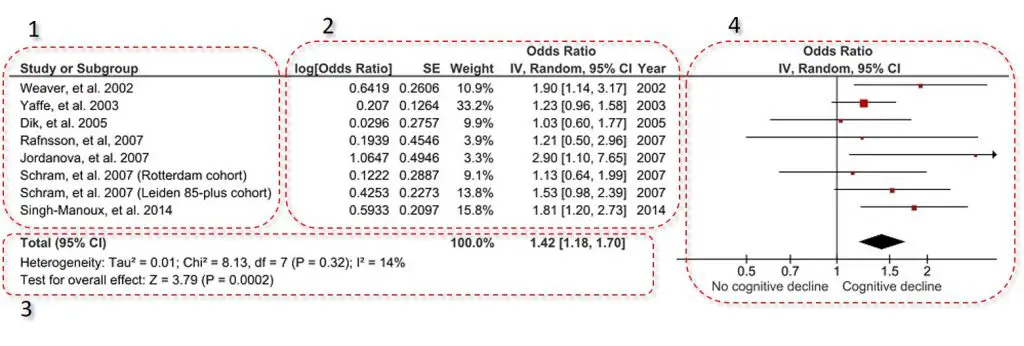
The included studies are usually placed in the far-left of the plot. This contains a list of the studies represented by the first author of the publication and the year it was published.

2. Effect estimate information

Next to the list of the included studies, are extra information on the studies effect estimates. In the example, the effect estimate measured were odds ratios (ORs). So the extra information was the log OR with the standard error (SE), as well as the actual OR and the 95% confidence intervals (CIs). This is the data which is plotted on the forest plot on the right.

Often found in this section is the study weight. The study weight is the power of the study. Generally, those studies which have lower variation, i.e. tighter 95% CIs or a higher n number, have a higher weight. Therefore, the higher the weight the more influence that study will have on the overall effect.

In this example, there is also an extra column titled Year. This lists the year of the included studies.

3. Overall statistics

Underneath the list of the included studies with their extra information is the overall statistics. Within this, there are two statistics presented: heterogeneity and overall effect.

Heterogeneity

The heterogeneity tests aim to determine if there are variations between the included studies, which may not be due to chance. Ideally, there should be zero heterogeneity between the included studies, thus indicating their suitability to be pooled into a meta-analysis. The test P value is quoted in brackets, in the example above this is ‘0.32‘, which would indicate no heterogeneity between the included studies.

Furthermore, RevMan includes the I 2 statistic. The I 2 statistic is presented as a percentage and represents the total variability in the studies effect measure which is due to heterogeneity. These values are often placed into three categories: no/low (<25%), moderate (25-50%) and high (>50%) heterogeneity.

Overall effect

The statistic of interest for a meta-analysis is the overall effect. In other words, when taking all of the included studies together, is the overall effect significant. In the example above, the overall effect P value is ‘0.0002‘, which indicates a very significant result.

4. Forest plot

This is the actual forest plot itself. I have annotated the example further below.

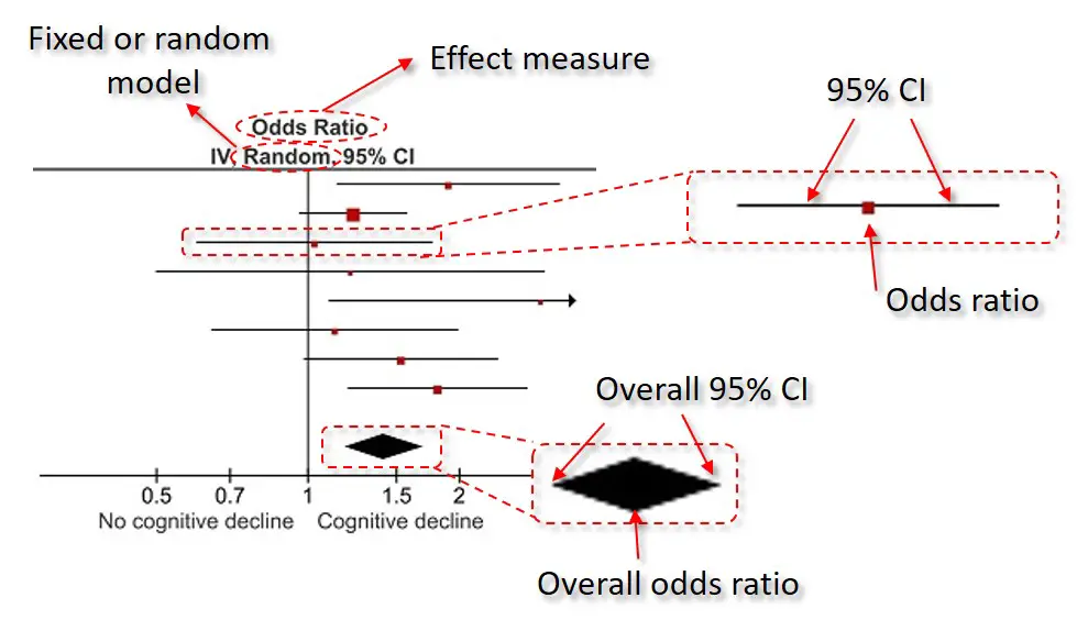
At the top of the plot, it will state the effect measure being plotted, in this case, odds ratios, as well as the type of model used (either a random- or fixed-effects model).

The plot itself contains the corresponding effect measure, indicated by a coloured dot, with the 95% confidence intervals (CIs) as whiskers. At the bottom, the overall effect measure is indicated by the middle of the diamond, with the 95% CIs at either side.

What is a forest plot?

A forest plot is a figure, frequently used in meta-analyses, which displays the results from similar individual studies stacked on top of one another with the overall summary measures at the bottom. Below is an example of a forest plot created using RevMan 5.

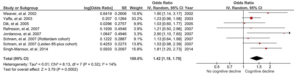
Forest plot is taken from Bradburn, et al. 2018.

Чтение лесного участка

Изучите личности

Исследования, включенные в метаанализ и включенные в лесной участок, обычно будут идентифицироваться в хронологическом порядке слева по автору и дате. Вертикальному положению, принятому в конкретном исследовании, не придается никакого значения.

Стандартизированная средняя разница

Часть диаграммы лесного участка будет справа и укажет среднюю разницу в эффекте между тестовой и контрольной группами в исследованиях. Более точное отображение данных отображается в числовой форме в тексте каждой строки, в то время как несколько менее точное графическое представление отображается в форме диаграммы справа. Вертикальная линия ( ось Y ) указывает на отсутствие эффекта. Горизонтальное расстояние прямоугольника от оси y демонстрирует разницу между тестом и контролем (экспериментальные данные с вычтенными контрольными данными) в отношении отсутствия наблюдаемого эффекта, иначе известного как величина экспериментального эффекта.

Усы доверительного интервала

Тонкие горизонтальные линии, иногда называемые усами, выходящие из рамки, указывают величину доверительного интервала . Чем длиннее линии, тем шире доверительный интервал и тем менее надежны данные. Чем короче линии, тем уже доверительный интервал и надежнее данные.

Если квадрат или усы доверительного интервала проходят через ось Y отсутствия эффекта, данные исследования считаются статистически незначимыми .

Масса

Значимость данных исследования или мощность указывается весом (размером) коробки. Более значимые данные, например, из исследований с большим размером выборки и меньшими доверительными интервалами, обозначены рамкой большего размера, чем данные из менее значимых исследований, и они в большей степени способствуют объединенному результату.

Неоднородность

Лесной участок может продемонстрировать степень, в которой данные нескольких исследований, наблюдающих один и тот же эффект, перекрываются друг с другом. Результаты, которые не могут хорошо перекрываться, называются неоднородными и упоминаются как неоднородность данных - такие данные менее убедительны. Если результаты разных исследований схожи, данные считаются однородными , и тенденция к тому, чтобы эти данные были более убедительными.

Неоднородность обозначена I 2 . Неоднородность менее 50% называется низкой и указывает на большую степень сходства между данными исследования, чем значение I 2 выше 50%, что указывает на большее несходство.

Пример

В этой блоббограмме используются семь исследований, чтобы показать, что кортикостероиды могут ускорить развитие легких при беременности, когда ребенок может родиться преждевременно . Отношение шансов (OR) одного указывает на отсутствие эффекта; исследования с доверительным интервалом (горизонтальные линии), пересекающим один (вертикальная линия), неубедительны. Мощные исследования (в данном случае с большим количеством участников ) имеют более узкие (более короткие) доверительные интервалы. Исследование с отношением шансов, равным единице, и очень узким доверительным интервалом не показало бы значительного эффекта. Здесь резюме и Оклендское исследование имеют узкие доверительные интервалы, которые не пересекаются с одним, что указывает на то, что эти исследования будут считаться статистически значимыми .

Эта капля взята из известного медицинского обзора ; он показывает клинические испытания на применении кортикостероидов для развития Спешите легкое в беременности , когда ребенок, вероятно, будет родиться преждевременно . Спустя долгое время после того, как было достаточно доказательств того, что это лечение спасает жизни младенцев, доказательства не были широко известны, и лечение не использовалось широко. После того, как систематический обзор сделал доказательства более известными, лечение стали использовать чаще, что предотвратило смерть тысяч недоношенных детей от респираторного дистресс-синдрома . Однако, когда лечение было развернуто в странах с низким и средним уровнем дохода, было обнаружено, что умирает больше недоношенных детей. Считается, что это может быть связано с более высоким риском заражения, которое с большей вероятностью убьет ребенка в местах с некачественной медицинской помощью. В текущей версии медицинского обзора говорится, что «нет необходимости» в дальнейших исследованиях полезности этого лечения в странах с более высоким уровнем доходов, но необходимы дальнейшие исследования о том, как лучше всего лечить матерей с низким уровнем дохода и с более высоким риском, и оптимальная дозировка.

Читайте также: